scPRINT
This post is just a paper summary scPRINT: a large cell model to predict and explain single-cell gene expression (Nature Communications, 2025), with code at github.com/cantinilab/scPRINT. What I want to do here is tell the story behind it — the design choices, the dead ends, the surprises, and the infrastructure we had to build.
If you prefer watching over reading, check out my talks at LoGG or at the scVerse community meeting.
Why scPRINT?
The backstory is in The PhD Decision, but the short version: existing foundation models for single-cell RNA-seq looked impressive on paper but were frustrating to actually use. scGPT had momentum, but the code was hard to extend, the reproducibility was shaky, and, perhaps most importantly, none of these models were actually designed to output gene networks. They mentioned it as a feature, but it was an afterthought.
Four things convinced me to build from scratch:
- The data is there, but it’s not being used well. CellxGene (CxG) had accumulated 50+ million cells from diverse species, tissues, diseases, and ethnicities. The existing models weren’t really leveraging this heterogeneity in a principled way.
- Zero-shot capabilities were largely absent. Models needed fine-tuning for nearly everything, which limits usability enormously — you can’t fine-tune on a dataset you haven’t seen yet.
- Gene network inference was essentially unmeasured. The “GRN inference” evaluations in previous papers used tiny networks, synthetic data, or methods borrowed from NLP attention analysis without biological validation.
- The infrastructure for network biology didn’t exist. You couldn’t store a gene network alongside single-cell expression data in any standard format. You couldn’t benchmark methods on a common suite of tasks. Both of these had to be built.
Building scPRINT
Starting from scratch (not from scGPT)
The initial plan was to start from scGPT and modify it. That plan died quickly. The codebase was not designed for the kind of changes we wanted to make, and the training pipeline had reproducibility issues we couldn’t work around. So we built scPRINT from scratch, which ended up being the right call — it gave us full control over every design decision.
Architecture: three tricks that matter
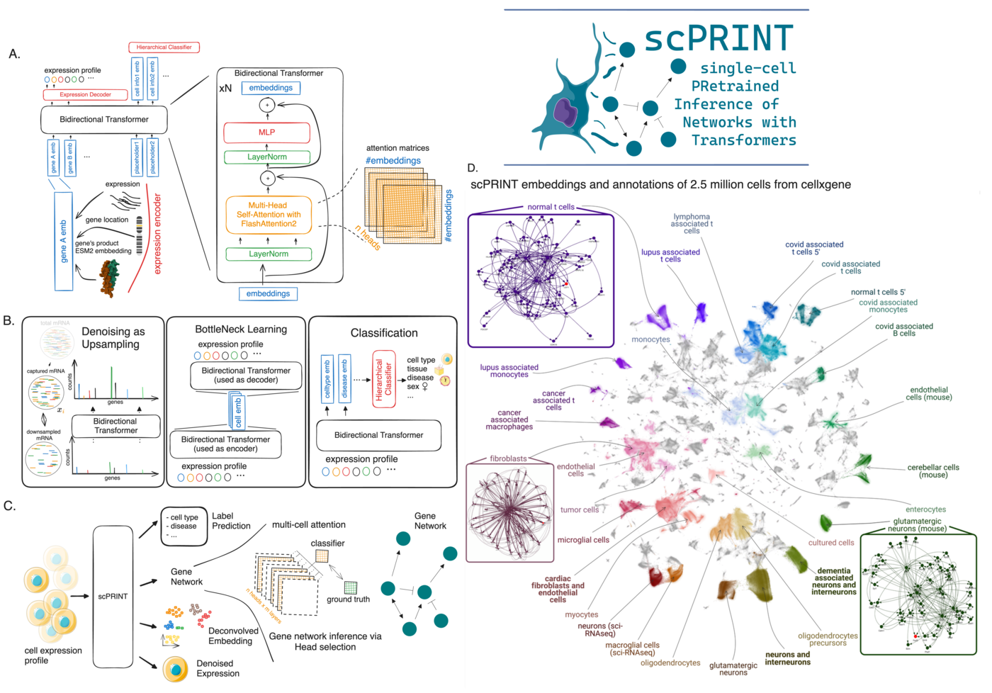
Gene tokens from protein structure, not a lookup table. scGPT and Geneformer use a learned gene embedding — essentially a vocabulary of ~30,000 genes, each with its own trainable vector. This works, but it creates a hard bottleneck: the model can only reason about genes it has seen during training, and the representation has no prior biological information baked in.
scPRINT instead encodes each gene using the ESM2 embedding of its most common protein product. ESM2 captures amino acid sequence and structural information trained on hundreds of millions of proteins. This means scPRINT inherits some protein-protein interaction priors from ESM2’s training, and — in principle — could generalize to unseen genes or species, because the representation is based on sequence rather than gene identity. First proposed in UCE, we extended this approach by combining it with expression tokenization and positional encoding.
Expression as a continuous quantity. Rather than discretizing expression levels into bins (as scGPT does) or ranking genes by expression (Geneformer), scPRINT feeds log-normalized counts through a small MLP. This lets the model learn its own metric over expression levels, rather than having us impose one.
Genomic position encoding. Genes that are close together on the chromosome tend to be co-regulated by the same DNA elements. We encode genomic location into each gene’s token, giving the model a spatial prior on gene-gene relationships.
Pretraining tasks: what we learned
The pretraining runs three tasks simultaneously, with their losses summed:
Denoising via upsampling. We randomly downsample 70% of a cell’s transcripts, then ask the model to reconstruct the full profile. This is more realistic than masking (which is what scGPT does) because it mimics the actual dropout structure of scRNA-seq data. It also gives scPRINT zero-shot denoising ability out of the box. One finding: including unexpressed genes in the input — padded with zeros — helps the model distinguish true biological zeros from dropouts. This sounds obvious in hindsight, but it wasn’t.
Bottleneck learning. The model generates a compact cell embedding, then uses only that embedding (without seeing the raw expression values again) to reconstruct the expression profile. This forces the embedding to be informative. It’s similar in spirit to how autoencoders work, but integrated into the transformer pretraining loop.
Hierarchical label prediction. Because CxG requires complete metadata annotations, we were able to add cell type, disease, sex, ethnicity, sequencing platform, and organism as prediction targets during pretraining. Each gets its own disentangled embedding: the first embedding learns to represent cell type, the second disease, and so on. This is unusual — most models treat labels as downstream fine-tuning targets rather than pretraining objectives — and it turned out to be important. The ablation study showed this consistently improves zero-shot performance, and the disentangled embeddings open up interesting future possibilities (counterfactual generation: mix “fibroblast” + “cancer” + “pancreas” embeddings to generate novel expression profiles).
One overall finding about training: the data quality and diversity is the real bottleneck, not model scale. We trained models from 2M to 100M parameters, and the gains from larger models plateaued before we exhausted the training data. The medium model (trained in 48 hours on a single A40 GPU) captured most of the performance. We made this efficiency a priority deliberately — a 48-hour training time means any computational biology lab can reproduce or fine-tune this work.
Gene Networks: the hard part
The most distinctive thing about scPRINT is that gene network inference is the primary objective, not a byproduct. Understanding what we actually did here — and why it was hard — requires stepping back.
The conceptual problem with GRNs
Gene regulatory networks have a branding problem. The name implies something clean and graph-like: nodes, directed edges, a tidy structure. The reality is messier. A cell is a complex dynamical system — thousands of molecular species interacting nonlinearly, with stochastic noise and context-dependence at every level.
Most GRN benchmarks up to this point had evaluated methods on networks of 10–50 hand-curated genes, defined using ODE-based simulators. That’s a tractable toy problem, but it’s almost entirely disconnected from genome-scale biology. We needed to ask: what would a meaningful genome-wide GRN even look like, and how would we evaluate it honestly?
Building the infrastructure
Two tools had to be created before we could even run experiments.
GRnnData is a lightweight extension of AnnData that treats gene networks as first-class objects. Standard AnnData stores expression matrices and cell metadata — but has no natural place for a gene×gene matrix associated with each cell type. GRnnData adds this, with efficient storage and slicing. If AnnData is the single-cell expression standard, GRnnData is the same for expression + networks.
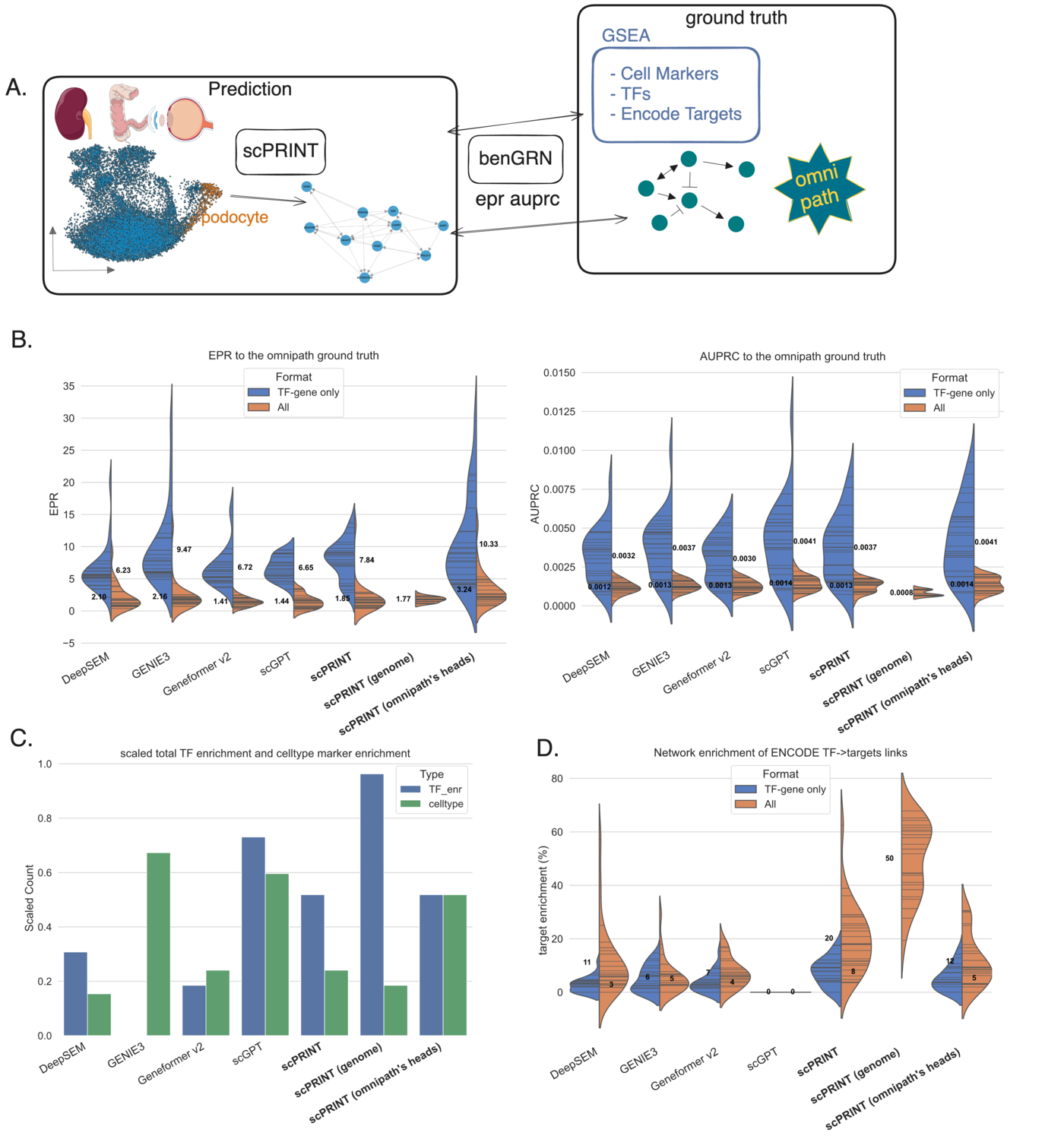
BenGRN is a benchmark suite with 4 tasks, 5 metrics, and multiple datasets covering different experimental contexts. Building this forced us to confront some uncomfortable truths about the field:
-
Z-scoring artifacts. Z-scoring expression data before network inference dramatically improves performance on the OmniPath ground truth, but hurts performance on perturbation-based benchmarks. Why? OmniPath contains many connections extracted from early cancer cell line array data, where housekeeping genes are co-expressed everywhere and generate spurious co-expression-based connections. Z-scoring aligns to that bias — not to biological truth.
-
The Geneformer attention trick. We found that aggregating Geneformer’s attention scores across many cells (rather than per-cell) substantially improves its network predictions. The reason: Geneformer only attends between genes expressed in the same cell, so summing across cells artificially inflates co-occurrence scores for genes that tend to be co-expressed. It’s correlation bias disguised as regulatory signal.
-
GENIE3 doesn’t scale. The standard GENIE3 setup — more cells, more trees — eventually produces runs that never finish on a cluster. We had to prune our benchmarks significantly just to make comparisons feasible. On genome-wide perturb-seq data, GENIE3 is competitive, probably because perturbation responses correlate somewhat with expression correlation, which GENIE3 is explicitly designed to exploit.
How scPRINT infers networks
scPRINT generates gene networks from its attention matrices — the same mechanism used in ESM2 for contact prediction in proteins. Each attention head captures a different pattern of gene-gene relationships. Not all heads are equally useful: in larger models especially, some heads become “unused” and contain mostly noise.
We address this with a head selection strategy: given a small subset of a ground truth network (OmniPath, ChIP-seq+perturb-seq intersections, or genome-wide perturb-seq), we train a linear classifier to find the combination of heads that best predicts those connections. Those same heads are then used for inference on all cell types. This is consistent — the same head combination applies across cell types and different subsets of the ground truth — and it’s transparent, unlike methods that aggregate all heads uniformly.
The result: scPRINT outperforms scGPT, Geneformer v2, DeepSEM, and GENIE3 on our atlas-level benchmarks. Key results:
- OmniPath recovery: scPRINT (omnipath’s heads) outperforms all methods. Even plain scPRINT outperforms scGPT and Geneformer on EPR (enrichment over random), meaning its top-ranked edges are more often true connections.
- ENCODE TF-target enrichment: scPRINT is the only method where a meaningful fraction (20%) of transcription factors have connections significantly enriched for their validated ENCODE targets. scGPT shows no enrichment across all 26 cell types tested.
- Cell-type-specific ground truths (MCalla et al., genome-wide perturb-seq): scPRINT outperforms all methods when head selection is applied. The result is particularly strong because these are direct, experimentally validated connections, not literature curation.
One counterintuitive finding: smaller scPRINT models (fewer attention heads) often perform better when averaging all heads. Larger models benefit more from head selection. This suggests that as models scale, attention specialization increases — some heads become highly informative, others become noise, and you need selection to isolate the signal.
Beyond Networks: Zero-Shot Capabilities
Because scPRINT’s pretraining is designed around a cell model — not just a gene-expression compressor — it develops zero-shot capabilities across several tasks that aren’t directly in its training objective.
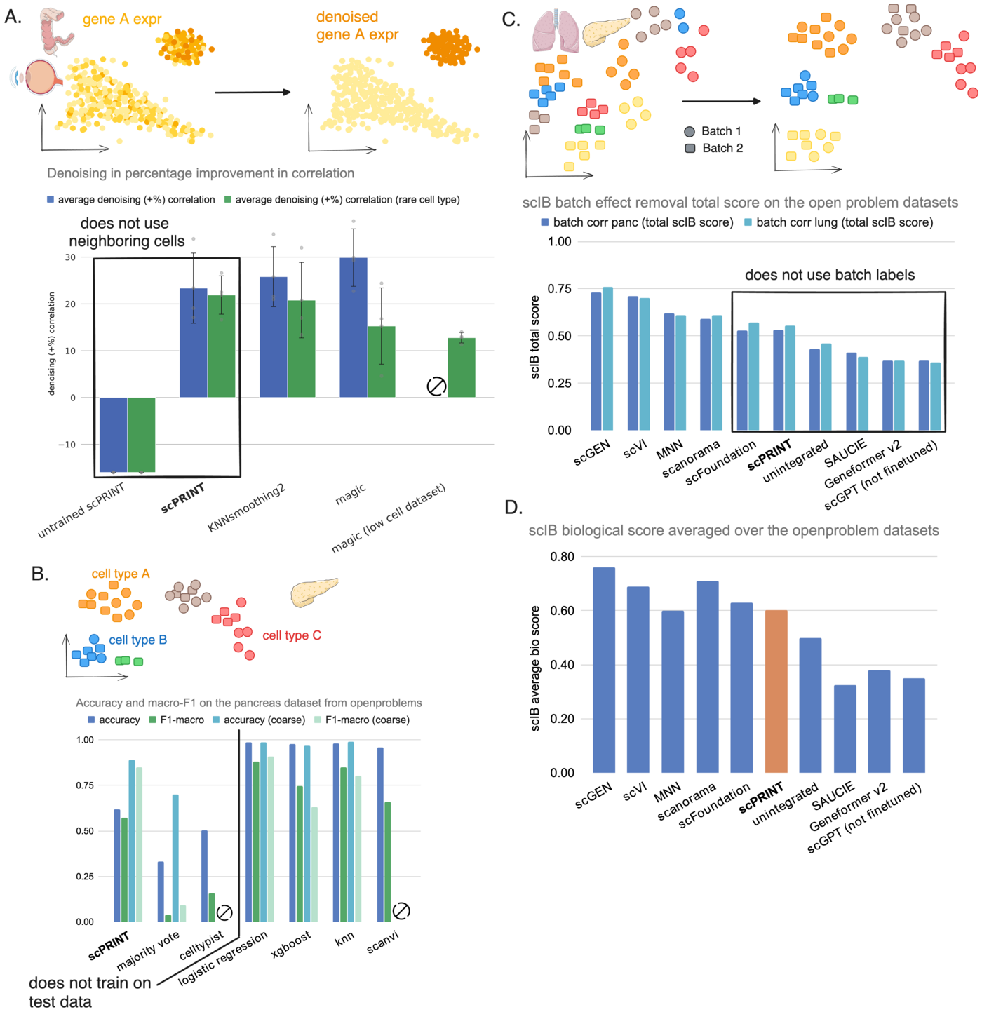
Denoising. On test datasets from CxG (ciliary body, colon, retina), scPRINT is competitive with MAGIC and KNNSmoothing2. But on rare cell populations (pericytes, microfold cells, microglial cells — 10 to 200 cells), scPRINT outperforms both substantially. Why? MAGIC and KNNSmoothing2 aggregate expression over neighboring cells, which breaks down when there are almost no neighbors of the same type. scPRINT operates independently over each cell, using learned gene-gene interactions rather than local cell-cell proximity.
Zero-shot cell type prediction. scPRINT predicts cell labels across 200+ cell type categories without seeing any labeled examples from the test dataset. At 62% accuracy, it substantially outperforms CellTypist (the most comparable zero-shot method). On macro-F1 — which weights all cell types equally regardless of frequency — it matches SOTA supervised methods like logistic regression and XGBoost, which have access to 70%+ of the test data for training. The one weakness: scPRINT struggles to distinguish closely related pancreatic cell subtypes (A, B, D, E cells). Using the coarser “endocrine” label, performance jumps dramatically.
Batch effect correction. Using its disentangled embeddings, scPRINT partially removes batch effects without using batch labels as prior information. On the OpenProblems lung and pancreas benchmarks, it achieves the top scIB score among all methods that don’t use batch label information. It doesn’t match dedicated integration tools like scVI or scGEN — which is expected — but it shows the cell model has learned to disentangle biological state from technical noise.
Application: Benign Prostatic Hyperplasia
To show that scPRINT does something useful in practice, we applied it to a prostate tissue atlas containing both normal and pre-cancerous (BPH) samples. scPRINT generated consistent batch-corrected embeddings across sequencers and age groups, annotated cell types with 71% accuracy, and identified rare cell populations in B-cells with early markers of tumor microenvironment.
In fibroblasts specifically, the gene network predicted by scPRINT recovered PAGE4 as a major hub — a known regulator linking senescence, ECM remodeling, and chronic inflammation. In BPH-associated fibroblasts, the network highlighted interconnected pathways of oxidative stress response and extracellular matrix building through metal and ion exchange — a non-obvious connection that points toward potential targets.
What I Would Do Differently
The GRN evaluation story is still incomplete. BenGRN is a real improvement, but the field lacks consensus on what a “correct” gene network even looks like at the genome scale. The three ground truths we used (OmniPath, MCalla, gwps) are substantially non-overlapping, which tells you something important: we don’t yet know what we’re measuring. I would push harder on this before the next paper.
Attention-based networks have limits. Using attention heads as a proxy for gene networks is principled but approximate. Attention captures pairwise gene relationships at a single layer, not causal structure across the whole network. I have ideas for how to go further, but they require architectural changes that scPRINT-2 begins to address.
The training data composition matters more than scale. We saw this empirically — more parameters did not help as much as better-curated training data. More work on filtering, weighting, and quality-controlling the CxG database would probably yield more gains than scaling to 500M parameters.
What Comes Next
Most of what I learned building scPRINT went into scPRINT-2. BenGRN and GRnnData are available if you want to use or extend them. Model weights and training code are public.
If you want to dig further:
- GitHub
- Nature Communications paper
- BenGRN benchmark
- GRnnData
- My GRN rant on X
- AUPRC vs AP discussion on X


Leave a comment