AUPRC vs AP: Evaluating Binary Classification

When analysing a classification task for my recent paper scPRINT, I fell into a fascinating “data-sciency” rabbit-hole about AUPRC, AUC and AP.

Understanding Classification Metrics

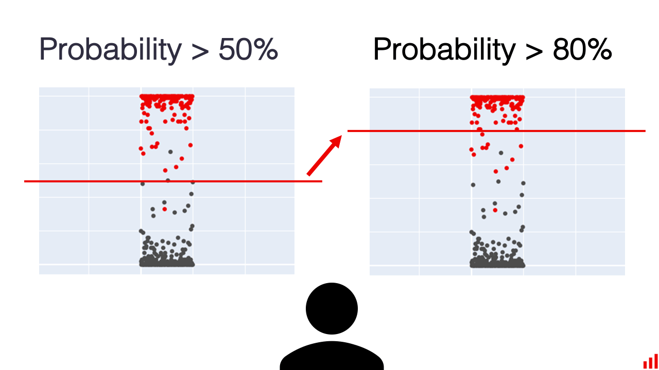
When evaluating a binary classification model that outputs probabilities or has internal regularization, we need ways to assess its performance across different decision thresholds.

ROC Curves

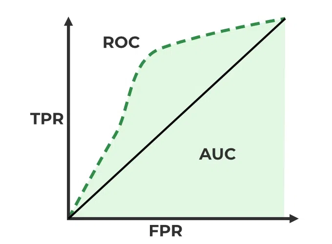
One common approach is plotting the ROC curve, which shows the tradeoff between true positive and false positive rates. The area under this curve (AUC/ROC-AUC/ROC/AUROC) is a popular metric:

The Need for Precision

However, in some cases like predicting graph edges in sparse gene networks, precision becomes crucial. AUROC can miss important information about optimal cutoff points. 🚫

AUPRC and Its Challenges

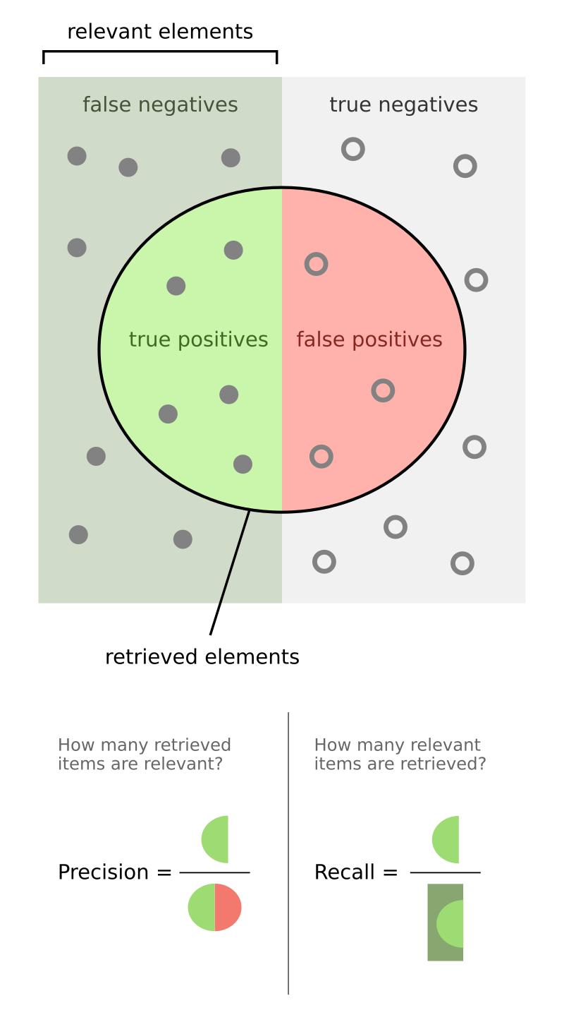
This is where AUPRC (PR-AUC) becomes valuable, focusing on precision and recall:

However, AUPRC comes with its own challenges: ⚠️

1. Random precision baselines differ between tasks, making direct comparisons difficult
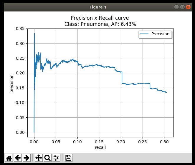
2. Jagged results require careful sampling of PR curves 😟
3. In gene network inference, many links lack prediction values, requiring special handling 🔥

Introducing rAUPRC

To address these limitations, I developed rAUPRC (random-baseline-corrected AUPRC), implemented in benGRN. It differs from vanilla AUPRC in three key ways:

1. Baseline correction — Standard AUPRC is heavily influenced by the positive class ratio. A dataset with 1% positives will have a baseline AUPRC of ~0.01, making comparisons across tasks meaningless. rAUPRC normalizes for this: a random classifier always scores 0, a perfect classifier scores 1, regardless of class imbalance. 🎯

2. Handling missing predictions — In gene network inference, most tools only predict a subset of possible links; the rest are simply absent (not predicted as negative). Vanilla AUPRC breaks here. rAUPRC handles this by treating missing predictions explicitly when drawing the recall axis, giving a fair picture even when coverage is partial. 🔍

3. Curve interpolation — PR curves are notoriously jagged, especially at low recall. rAUPRC uses a modified interpolation that avoids the artificial inflation that naive linear interpolation can introduce between operating points.

In practice on GRN benchmarks, rAUPRC produced more stable rankings across different network densities and prediction tool outputs than either vanilla AUPRC or AP. 📊

Average Precision (AP)

AP is computed as:

AP is a discrete approximation of AUPRC — rather than integrating the continuous curve, it sums precision at each threshold where a positive is retrieved, weighted by the change in recall:

\[AP = \sum_n (R_n - R_{n-1}) \cdot P_n\]

In practice, AP and AUPRC give very similar values when the PR curve is sampled densely. The key difference is that AP is purely a summary statistic (one number per run), while AUPRC can be computed from the full curve and lends itself better to baseline correction.

AP is often recommended for object detection and ranking tasks (it’s the default in PASCAL VOC and COCO benchmarks). For gene network inference and other sparse biological tasks, rAUPRC is more appropriate. ✅

When to use what

Metric	Use when
AUROC	Classes are roughly balanced, you care about ranking overall
AUPRC / AP	Strong class imbalance, precision matters
rAUPRC	Gene networks, partial predictions, cross-task comparison

For a deeper dive into the implementation, see the benGRN repo and the benchmarking section of the scPRINT paper.