DepMap Omics: How to

The goal of this blog post is to explain how to run the DepMap omics pipeline as our brave Associate Computational Biologist do.

Introduction

Large panels of comprehensively characterized human cancer models have provided a rigorous framework with which to study genetic variants, candidate targets, and small-molecule and biological therapeutics and to identify new marker-driven cancer dependencies.

As part of its discovery effort of Cancer Dependencies an Targets, DepMap analyzes raw omics data from cell lines on a quarterly basis. This part of the project if often referred to as CCLE. The bulk of ccle data consists of many omics sequences as shows in the CCLE2 paper. However only RNAseq and Whole Exome seq gets generated and analyzed quarterly. This project is lead by a team of researchers from the CDS group at the Broad Institute and draws from other projects such as GTeX, TCGA and CCLF.

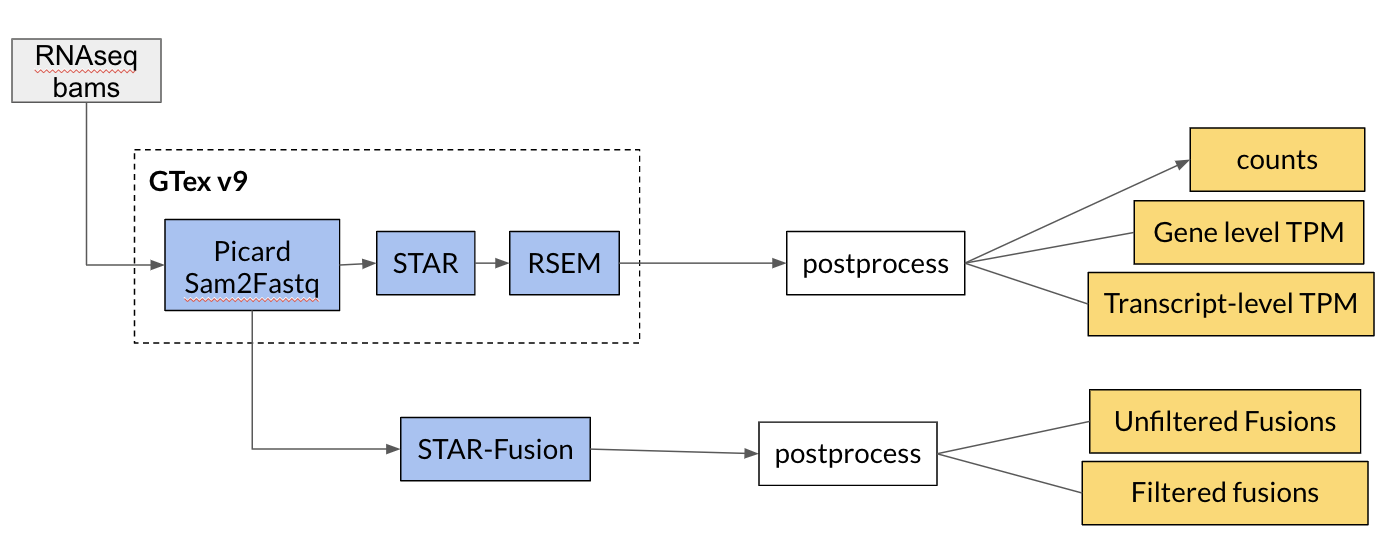
RNAseq pipeline

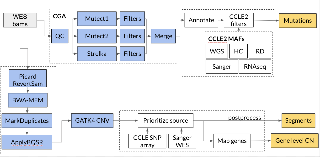
WES pipeline

The following tools are used in our pipelines:

• star:
  • https://www.ncbi.nlm.nih.gov/pubmed/23104886
  • https://github.com/alexdobin/STAR/blob/master/doc/STARmanual.pdf
• rsem:
  • https://bmcbioinformatics.biomedcentral.com/articles/10.1186/1471-2105-12-323
• star fusion:
  • https://github.com/STAR-Fusion/STAR-Fusion/wiki
  • http://biorxiv.org/content/early/2017/03/24/120295
• mutect:
  • https://software.broadinstitute.org/cancer/cga/mutect
  • https://youtu.be/rN-cLrb5aGs
  • https://software.broadinstitute.org/gatk/documentation/tooldocs/4.beta.4/org_broadinstitute_hellbender_tools_walkers_mutect_Mutect2.php
  • https://www.nature.com/articles/nbt.2514
• gatk cnv:
  • https://software.broadinstitute.org/gatk/documentation/article?id=11682
• strelka:
  • https://www.nature.com/articles/s41592-018-0051-x
  • https://github.com/Illumina/strelka

Furthermore the pipelines make use of several software development tools. In particular some familiarity with the following tools are recommneded:

• python
• R
• jupyter
• WDL
• gcp
• docker
• Terra
• dalmatian
• Terra and gcp

Why

Knowing how to run these pipelines will help you if you want to:

1. run your own large scale multi omics analysis pipeline. #Fancy
2. if you want to reprocess some of DepMap-omics sequencing in the same way it has been done to generate what is available on depmap.

The next sections are a detailed walkthrough to run DempMap omics pipelines on the Terra platform.

Installation

clone the required repositories

This repo uses some important data and code from the JKBio Library custom repositories. This repository and the ccle_processing one should be cloned into the same path using the following command:

git clone https://github.com/broadinstitute/ccle_processing.git
git clone https://github.com/jkobject/JKBio.git

You will need the approriate R packages and python packages

note that up to date versions are recommended

1. You will need to install Jupyter Notebook and Google Cloud SDK
   • install Google Cloud SDK.
   • authenticate your Google account by running gcloud auth application-default login in the terminal.
2. For R packages, a loading function contains most required ones (in here)
3. install the following additional R packages using the provided commands:
   • Another R package needs to be installed like so: cd src/cdsomics && R CMD INSTALL . && cd -.
   • And Celllinemapr: cd ../JKBio/cell_line_mapping-master/celllinemapr && R CMD INSTALL . && cd -.
4. For Python use the requirements.txt file pip install -r requirements.txt.

Creating your Terra Workspaces:

How to create workspaces and upload data to it is explained in Terra’s documentation

For the specific workflow ids, parameters and workspace data you can use the file data/xQx/.json in our ccle_processing repository, which lists the parameters used for each workflow of each off the 3 workspaces in our pipelines for each releases (the .csv file lists the workflows with their correct name): In order to have a working environment you will need to make sure you have:

• set a billing account
• created a workspace
• added the correct workspace data to it (the workspace parameters/data listed in the GENERAL field of the json file)
• imported the right workflows (in the csv file)
• parametrized them (in the json file)
• imported your data (Tools available in TerraFunction in the JKBio package as well as the dRalmatian package can be used to automate these processes.)

Once this is done, you can run your Jupyter Notebook server and open one of the 3 \*_CCLE Jupyter files in the ccle_processing repo, corresponding to our 3 pipelines.

• RNAseq processing of gene level and transcript level read counts and exon counts.
• WESeq processing of Copy Number (gene level and segment level)
• RNAseq & WESeq processing of Mutations (cancer drivers and germlines)

These notebooks architecture is as follows:

1. Uploading and pre-processing
2. Running the Terra Pipelines
3. Downloading and post-processing
4. QC, grouping and uploading to the portal

Running the notebooks

Each Following steps correspond to a specific part of each of the 3 notebooks.

Note that you can try it out using our publicly available bam files on SRA

1. Uploading and pre-processing

You can skip this step and go to part2.

The first step in the notebook is about getting the samples generated at the the Broad Institute which are located in different Google Cloud storage paths. This section also searches for duplicates and finds/adds the metadata we will need in order to have coherent and complete sample information.

Remarks:

• in the initialization step you can remove any imports related to taiga and gsheet to avoid possible errors.
• feel free to reuse createDatasetWithNewCellLines, GetNewCellLinesFromWorkspaces or any other function for your own needs.

2. Running Terra Pipelines

Before running this part, you need to make sure that your dalmatian workspacemanager object is initialized with the right workspace you created and that the functions take as input you workflow names. You also need to make sure that you created your sample set with all your samples and that you initialized the sampleset string with its name You can then run the pipeline on your samples. It would approximately take a day to run all of the pipelines.

Remarks:

• for the copy number pipeline we have parametrized both an XX version and an XY version, we recommend using the XY version as it covers the entire genome
• for the mutation calling pipeline we are working on Tumor-Normal pairs which explain some of the back and forth between the two workspace data table (the existing workflows work with or without matched normals).
• for the expression pipeline, we have an additional set of workflows to call mutations from RNAseq, this might not be relevant to your need.

3. Downloading and post-processing (often called 2.2-4 on local in the notebooks)

This step will do the following tasks:

• delete large intermediary files on the workspace that are not needed
• retrieve from the workspace interesting QC results.
• copy realigned BAM files to a target bucket.
• download the results.
• remove all duplicate samples from our downloaded file (keeping only the latest version of each samples).
• saving the current pipeline configuration.

You will at least need to download results, but other steps could be useful for some users

Post-processing tasks

Unfortunately for now the post-processing tasks are not all made to be easily run outside of the CCLE pipelines. Most of them are in R and are run with the Rpy2 tool.

So amongst these functions, some of them might be of a lesser interest to an external user. The most important ones for each pipelines are:

• processSegments
• interpolateGapsInSegmented
• extendEndsOfSegments
• generateEntrezGenes

• generateGeneLevelMatrixFromSegments

• readMutations
• createSNPs
• filterAllelicFraction
• filterMinCoverage you would need to rewrite this function as it now runs on DepMap columns. In one line it requires that the total coverage of that site (aggregated across methods) > 8 and that there are at least 4 alternate alleles for each mutations
• maf_add_variant_annotations

• mutation_maf_to_binary_matrix

• readTranscripts
• readCounts
• readTPM
• readFusions
• filterFusions
• the step 2.2.5 where we remove samples with more then 39k transcripts with 0 readcounts.
• prepare_depmap_\*\_for_taiga

Remarks:

• in the RNAseq pipeline we have an additional sub-pipeline at the end of the notebook to process the fusion calls from STAR-Fusion.
• to get the exact same results as in CCLE, be sure to run genecn = genecn.apply(lambda x: np.log2(1+x)) to produce the genecn dataframe in the CNV pipeline (present at the end of the validation steps).
• we do not yet have integrated our germline calling in the mutation pipeline but you can still find the haplotypeCaller|DeepVariant workflows and their parameters

4. QC, grouping and uploading to the portal

These tasks should not be very interesting for any outside user as they revolve around manual checks of the data, comparison to previous releases, etc.

In these tasks we also prepare the data to be released to different groups, removing the samples per access category: Blacklist|Internal|DepMapConsortium|Public. We then upload the data to a server called taiga where it they be used by the DepMap portal to create the plots you know and love.

You can however find all of these files directly on the download section

---

you can find the project’s repository here the blog post is available on depmap’s blog and Jérémie’s blog

Please feel free to ask any question on our FAQ

Jérémie Kalfon