UMAP: Uniform Manifold Approximation and Projection for Dimension Reduction

Umap is a dimensionality reduction algorithm. It takes points defined by vectors of high dimensions:

• 2D vector= (x,y),
• 3D vector= (x,y,z),
• ND vector= (x,y,z,a,b,c,…n)

And puts them back in lower dimensions. This allows for visualizing point clouds in 2D and also finding a subspace/ base / manifold in which the cloud data lies.

This can be better seen in the 3D to 2D case. The reduced vector is also called an embedding of the first one.

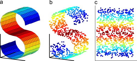
View of learning the shape of a “sheet of paper” only by knowing a set of points that lie on it.

Unlike many other famous techniques (PCA, MDS…), it learns this structure by using local information. i.e. only looking at specific patches at a time. The neighbors of each points, like t-SNE. This type of technique is called non linear as it can learn complex “bendy” shapes (like the S above).

Neighbor information is better encoded into a graph. With edges representing distances between points. and only displaying the edges to the nearest points in the neighborhood.

This distance is normalized by all distances this point has to its neighbors, meaning now the range of possible distances is transformed into a [0,1] range where the closest point will be at a distance 0 and the furthest point will be at a distance computed such that summing all the distances between all neighbors will get to $log2(#neibors)$.

Then for all the neighbors we create a set (a list of unique things) for all edges.

This set will be “fuzzy”, as it also contains a value representing how much each neighbors to a point is in the set of neighbors to this point, based on its distance to the center point.

We will do this for each point and then merge all the sets created for each point. Meaning, we will merge the edges and keep only the ones with the lowest distances.

We then take each edges and consider them together as a graph or a skeleton.

Pausing for a second, we can really see that the only thing we have done here is defined edges between points and merging them together. However you have to understand that the same edge in two different set, will have two different distances as they have both been normalized by different sets of neighbors. Thus even a point far away from everything else will get one of its edges in the graph. These two edges would get merged by using the t-conorm (which a fuzzy logic way of taking the norm of something) on their two respective lengths.

Note that we are thinking here about graph of nodes and edges but the topological logic could be applied to the faces made by each set of 3 edges and the volumes made by each set of 4 faces, etc … This would complexify the model (and render it impossible to compute) but also make it more closer to the theory underlying it

We then take the core components of this graph using spectral embedding, where we basically take the eigenvector of a matrix of adjacency (i.e. A square of numbers where rows represent the nodes of the graph and the columns represent the same nodes and the values of the matrix are the distance between, each point)

It is a decomposition of the information into two things: one that define a base for the object to exist in and the other defining the layout of the object. You need both to reconstruct the object.

Here we will only take the first 2 most important value of the base and considers it as what defines our object in 2 dimension (but it could be any other number, lower than the initial number of dimension). The two values here are vectors: they represent the 2 dimensions of each points (x,y) and each of their value/dimensions represent each of the different points in our point cloud.

Finally we will try to improve this first version by a minimization process. There, we want to apply a physical-like force between the nodes so that close connected edges get closer together (up to a minimum distance)

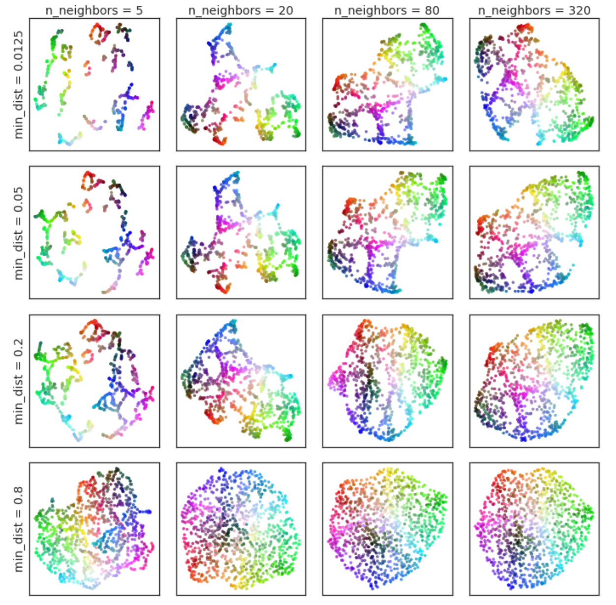
we can see the relation to the number of samples used and the max distance to create graph edges.

All in all, there is a theoretical explanation of the algorithm that can be seen in terms of learning fuzzy simplicial sets defining the local structure of the high dimensional data and of the lower dimensional one and making the two sets converge.

The explanation defined in part 2 of the paper can be understood by anyone after reading this book which will allow the reader to gain the vocabulary to understand the wikipedia pages defining the vocabulary used in the paper. :p

More information about Riemannian topology can then be learned here. It is in French however ;)