Most of the time, even when textbooks go into molecular detail, the story is still organized around dogmas. One chapter adds chromatin. Another adds transcription factors. Later, RNA processing appears. Then translation, protein degradation, signaling, condensates, non-coding RNAs, and so on. Each new mechanism is real, but they often arrive as separate layers of complexity, not as one formal picture of what we collectively know.

That is what I tried to build here: a summary of our current formal knowledge of gene regulation, placed into one landscape.

While doing it, I noticed something that surprised me. Biology has many measurements and many local names, but sometimes no clean conceptual object for things that are probably views of the same underlying cellular structure. For example, super-enhancers in ChIP-seq and transcriptional condensates in microscopy are not strictly identical, but they are clearly not unrelated either. In other places, molecular biology has long descriptive sentences for mechanisms, but no short handle that makes the mechanism easy to reason about.

So I gave each main mechanism a short code name. The names are not meant to replace the biology; they are handles that point back to precise glossary entries. I hope the map is useful, and maybe sparks discussions.

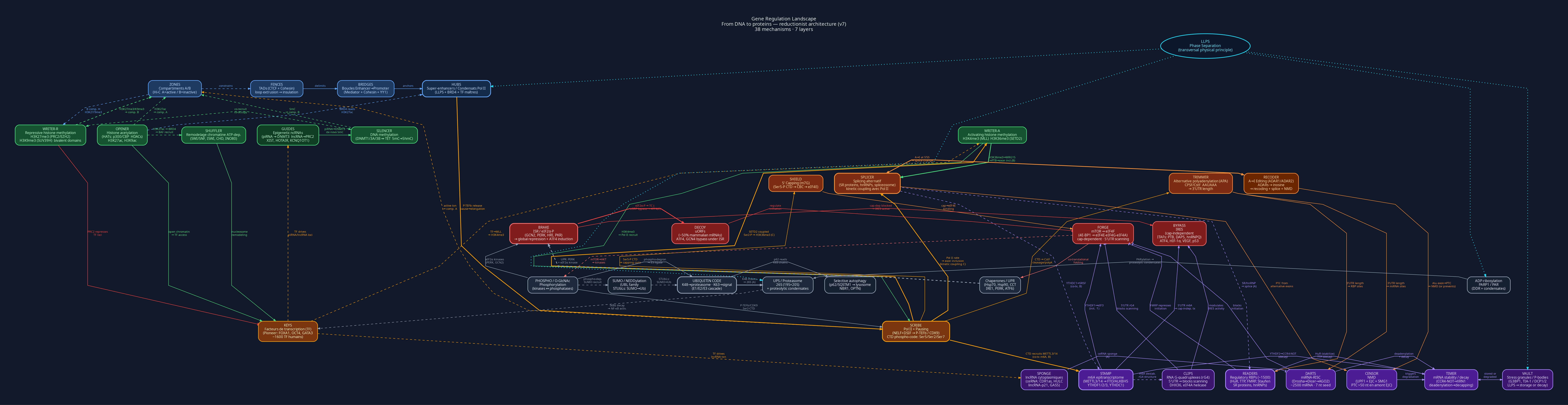
The map is very large, so the embedded version below is mostly a preview. You can open the full-resolution zoomable map here. The companion technical notes contain the 1-to-1 glossary for every box name, the full mechanism catalogue, link rationale, and legend details. The Graphviz DOT source is also available. A node-by-node literature audit now reviews the biological support, caveats, and proposed graph revisions for all 37 mechanism boxes. Several arrows were added or softened after that audit: for example, the cap now links to mRNA stability, growth and translation state now regulate decoding tempo, codon optimality and translation surveillance now link to mRNA decay, chaperone triage links back to ubiquitin routing, signaling links to CRL licensing, and nuclear lncRNA guides link to repressive histone writers. Other arrows are deliberately dashed because the evidence is contextual rather than universal.

In the figure, each box title is a code name that maps 1-to-1 to the catalogue entry in the technical notes. Solid arrows are the main mechanistic relations; dashed arrows indicate contextual, feedback, or association-style links; tee-headed arrows indicate repression; bold arrows mark especially important coupling edges. Border styles mark meta-principles such as LLPS and DECAY: these are recurring physical or regulatory motifs that appear across several mechanisms, not separate boxes in the pathway.

The map is also intentionally reductionist. I did not try to draw every important named event as its own box. Some biological phenomena are real and important, but they are better understood as outputs of several lower-level mechanisms already shown in the graph. For example, promoter/TSS choice depends on transcription-factor grammar, chromatin accessibility, enhancer contacts, and Pol II initiation/pausing. Transcription termination depends on Pol II state, cleavage/polyadenylation, chromatin context, and RNA decay machinery. Whether an RNA leaves the nucleus depends on capping, splicing, 3’ processing, RNA-binding proteins, RNA marks, and quality control. In those cases, the goal is not to add a new named event whenever biology has a label for one. The goal is to ask whether the underlying decision mechanisms and their links are already represented.

This is also why some familiar topics, such as R-loops, DNA torsional stress, transcription-replication conflicts, nuclear bodies, broad epitranscriptomic marks beyond m6A, repeats/transposons, motif grammar, and Pol I/Pol III rRNA/tRNA biology are handled as caveats, extensions, or submechanisms in the technical notes rather than as new boxes in the main landscape. That choice is not a claim that they are unimportant. It is a claim about map resolution: this figure prioritizes reusable regulatory mechanisms over named composite events.

Post-translational control is shown with representative feedback routes rather than every substrate-specific event. SWITCH, ROUTER, and DESTROY can touch many upstream programs; the map draws the main recurring routes to TF activity, Pol II, stress translation, proteostasis, and mTOR/NF-κB-style feedback. LICENSE is intentionally narrower: NEDDylation mainly activates cullin-RING E3 ligases, so its main graph role is to feed ROUTER.

Box Glossary

Each box in the image has exactly one entry here. Box titles are the short code names; italic text inside the image marks genes or proteins when the label needs examples.

Term Glossary

These are the main non-gene, non-protein terms used in the figure and glossary.

The Seven Layers

The map follows the flow from DNA to RNA to protein:

1. 3D genome: ZONES, FENCES, BRIDGES, and HUBS represent A/B compartments, TADs, enhancer-promoter loops, and super-enhancers that can overlap with transcriptional condensates without being identical to them.
2. Epigenetics: SILENCER, OPENER, WRITER-A, WRITER-R, SHUFFLER, and GUIDES cover DNA methylation, histone marks, chromatin remodeling, and non-coding RNAs that guide chromatin complexes.
3. Transcription: KEYS are transcription factors; SCRIBE is Pol II, promoter-proximal pausing, and the phosphorylation code of its CTD.
4. Co-transcriptional processing: SHIELD, SPLICER, TRIMMER, and RECODER cover capping, alternative splicing, alternative polyadenylation, and A-to-I RNA editing.
5. Post-transcriptional control: STAMP, READERS, DARTS, SPONGE, CENSOR, TIMER, CLIPS, and VAULT cover m6A, RNA-binding proteins, miRNAs, lncRNAs, nonsense-mediated decay, mRNA stability, RNA structures, and cytoplasmic granules.
6. Translation: FORGE, BRAKE, DECOY, BYPASS, TEMPO, and INSPECTOR describe cap-dependent initiation, the integrated stress response, uORFs, non-canonical initiation, decoding kinetics, and ribosome quality control. TEMPO now also folds in decoding fidelity: recent proteogenomics across >1,000 human samples found thousands of non-genomic amino-acid substitutions from alternate ribosomal decoding — not explained by DNA variants or A-to-I editing — producing proteoforms that are stable, abundant, and tissue/cancer-specific (Tsour et al., Nature 2026). Because these proteins partly escape INSPECTOR surveillance and persist into MATURE, this belongs on the speed-vs-fidelity axis of TEMPO rather than in RECODER (which is transcript-level A-to-I editing).
7. Post-translational regulation: SWITCH, ROUTER, TETHER, LICENSE, DESTROY, MATURE, and PAR cover phosphorylation/O-GlcNAc, ubiquitin, SUMOylation, neddylation, proteasome/autophagy clearance, maturation/UPR, and PARP/PAR signaling.

Across the whole diagram, border styles flag recurring meta-principles. LLPS marks liquid-liquid phase separation, and DECAY marks turnover or clearance. They are not extra regulatory layers. They are reused in several places: transcriptional condensates, stress granules and P-bodies, mRNA decay, proteolytic condensates, autophagy, and DNA damage repair assemblies.

The Useful Reduction

The full map contains 37 mechanism boxes, 2 meta-principles, and dozens of interactions. But conceptually, most of gene regulation reduces to three strategies.

1. Control accessibility.
Make a substrate accessible or inaccessible to its molecular machinery. Chromatin opening lets transcription factors bind. TADs constrain which enhancers can contact which promoters. Stress granules temporarily remove mRNAs from translation. miRNAs and lncRNAs tune whether an mRNA is available to the ribosome.

2. Write a reversible mark, then interpret it.
Histone methylation, DNA methylation, m6A, phosphorylation, ubiquitination, SUMOylation: the mark alone is never the full story. The reader and the context determine the output. m6A can promote translation or accelerate decay. A K48 ubiquitin chain points toward the proteasome; K63 often acts in signaling or selective autophagy. Phosphorylation can activate a transcription factor or create a degron.

3. Couple two processes through kinetics.
Some regulation is not a static state but a timing problem. Pol II elongation speed influences exon choice. SETD2 deposits H3K36me3 during elongation, linking transcription to splicing. eIF2α phosphorylation globally slows translation but selectively favors ATF4 through uORF logic. Codon usage changes ribosome speed and can influence co-translational folding.

That is the central idea of the landscape: gene regulation is not just a list of mechanisms. It is a multi-layer control architecture built from recurring design patterns.

Why This Matters For AI Biology

For AI biology, this kind of map is not only educational. It shows why predicting “gene expression” cannot be reduced to reading a promoter sequence.

The output of a gene depends on chromatin state, 3D contacts, Pol II kinetics, splicing, RNA modifications, RNA-binding proteins, translational control, and protein lifetime. A model that wants to predict perturbation response, cell state, or disease mechanism needs to represent at least part of this stack.

The lesson of the Gene Regulation Landscape is simple: gene expression is not a scalar. It is the endpoint of a control system.

Sources To Anchor The Map

• Core & Adelman, 2019, promoter-proximal Pol II pausing: https://pubmed.ncbi.nlm.nih.gov/31123063/
• Naftelberg et al., 2015, transcription/chromatin/splicing coupling: https://pubmed.ncbi.nlm.nih.gov/26034889/
• Wang & He, 2014, dynamic RNA modifications: https://pubmed.ncbi.nlm.nih.gov/25263552/
• Wang et al., 2015, m6A and translation efficiency: https://www.cell.com/cell/fulltext/S0092-8674(15)00562-0
• Shi et al., 2017, YTHDF3 translation/decay: https://pmc.ncbi.nlm.nih.gov/articles/PMC5339834/
• Sabari et al., 2018, coactivator condensation at super-enhancers: https://pmc.ncbi.nlm.nih.gov/articles/PMC6092193/
• Robson et al., 2019, chromatin topology: https://pubmed.ncbi.nlm.nih.gov/31324893/

I started in October 2023. Took 2.5 years instead of two. Here’s what happened.

What I set out to do

The project was building foundation models for single-cell transcriptomics — taking the pretraining ideas from NLP and applying them to gene expression at scale. The goal: a model that could infer gene regulatory networks, classify cell types zero-shot, denoise expression, and actually be useful to biologists. Not just publishable, usable.

%% WIP$$$

I was split between two labs: Laura Cantini at Institut Pasteur (computational biology, gene networks) and Gabriel Peyré at ENS (applied mathematics, optimal transport). Two very different worlds, two sets of expectations, two weekly meetings.

Outside the lab, I wanted to keep training — endurance sports had become important to me during this period, and I wanted to see more of the world while I could.

What I did

The papers

The thesis produced three papers:

scPRINT (Nature Communications, 2025) — a large cell model trained on 50M+ cells for gene network inference. Novel gene tokens from ESM2 protein embeddings, learned expression tokenization, genomic positional encoding. State-of-the-art on GRN inference benchmarks, zero-shot cell type classification, denoising. Code at github.com/cantinilab/scPRINT.

Xpressor — a cross-attention architecture for learning across biological scales. The idea: compress gene-level representations into cell-state vectors, and fine-tune protein language models using cellular tasks. Improved cell-type prediction (+28%) and embedding quality (+8%) over standard architectures.

scPRINT-2 (in revision, Nature Methods) — trained on 350M cells from 16 organisms, 25 TB of data. 42-model ablation study to figure out what actually matters in scFM design. 75% zero-shot cell type classification on OpenProblems (up from 47% with scPRINT-1). State-of-the-art denoising, batch correction, cross-species generalization, counterfactual generation.

The tools

Seven Python packages released: scPRINT, BenGRN (GRN benchmarking), GRnnData (gene networks in AnnData), and more for data processing, evaluation, and model serving. Everything open-source under GPL-v3.

The conferences

Over a dozen conferences and workshops across Europe and beyond. Oral presentations, poster sessions, invited talks. Each one forced me to sharpen the story and meet people working on adjacent problems.

The outreach

I mentored a student during the PhD. Wrote blog posts (you’re reading one), made videos, gave talks to non-specialist audiences. I think this kind of work matters — it’s how ideas spread beyond the 50 people who read your paper.

The people

The labs at Pasteur and ENS. Jules Samaran, Remi Trimbour, Geert Huizing at ENS. Alex Wolf, Sergei Ribakov, Brice Rafestin for software help. The Nucleate community, Whitelab Genomics, Blossom, dot Omics, Biographica. A lot of people made this work possible.

Outside the lab

I trained for and ran a medium triathlon, a half-marathon, the Mont-Blanc trail, and the Paris Marathon. Traveled to the UK, Portugal, Spain, Guadeloupe, Vancouver, Thailand. I needed this. Long runs are good for thinking, and getting away from the screen makes you come back sharper.

The defense

March 25. Pasteur, Duclaux amphitheater.

I was stressed. I’d prepared well, but defending years of work in one afternoon is a strange exercise. You try to make it look like everything was planned from the start, when in reality half of the good ideas came from accidents.

The jury was rigorous but fair. Hard questions in the Q&A — the kind that make you think, not the kind designed to trip you up. That’s what makes a defense feel worth it.

Having my mentoree there meant a lot. And the next week, I finished a marathon. Different kind of endurance, same feeling at the end.

What I learned

How to write papers. How to think about research impact beyond citations. How to set goals when nobody is setting them for you.

The research community matters more than I expected. Not just for collaboration — for sanity. The conferences, the DMs, the random conversations at poster sessions. Open source is how you actually have an impact: if scPRINT is useful, it’s because people can use it.

Technically: a lot about transformers, diffusion models, optimal transport, the math of self-supervised learning. But also about the gaps — the missing data, the incomplete benchmarks, the things we still don’t know how to measure properly.

Company research and a PhD are different. The PhD gave me time to go deep, be wrong for months, follow a thread until it broke or became a paper. I wouldn’t trade that.

What’s next

I’m not going back into academia. Never planned to. 🚀

I’m thinking of building Jouvence — a company using AI and biology to extend healthy human lifespan. The thesis work on foundation models, gene networks, and cellular representation is directly relevant: if you can model how cells work and how they break, you can start to intervene.

I’m also looking at companies working on similar goals: longevity, disease modeling, AI-driven high-throughput data generation. Places like Lilas Bioscience and Xaira Therapeutics are doing interesting work in this space.

Lots to do.

The full arc: the PhD decision, a year in, and now this.

Thanks to Laura, Gabriel, Juliette, my family, and everyone who was part of the last 2.5 years.

To train a cell foundation model that actually generalizes, you need thousands of datasets. You need to find them, download them, harmonize gene names across species, align cell type labels to controlled ontologies, preprocess everything consistently, store it in a way that doesn’t collapse under its own weight, and feed it to a model at scale. Managing a dozen datasets is already painful for most computational biologists. I needed to handle thousands.

Thirty months ago, three things came at exactly the right moment. The Chan Zuckerberg Initiative had made around 700 datasets easily accessible through CellxGene. The LaminDB project gave me a way to manage large, heterogeneous collections of biological data with metadata that actually meant something. And Sergei Rybakov was building a loader for streaming single-cell data at scale.

Managing scale with LaminDB

The core problem with large-scale single-cell data is not raw file size. It’s the metadata. A dataset from a 2019 mouse lung study uses different gene IDs, different tissue labels, and different cell type annotations than a 2023 human heart study. Reconciling these across hundreds of datasets by hand is a losing battle that compounds as the corpus grows.

LaminDB treats biological ontologies as first-class citizens. Every dataset I ingested was linked to standardized terms: Cell Ontology for cell types, Uberon for tissues, NCBI Taxonomy for species. That ontological consistency is what made it possible to build scPRINT-2’s hierarchical classification loss, which penalizes predictions based on their distance in the ontology graph rather than just correct/wrong. The loss knows that “T cell” and “CD8-positive T cell” are related in a way that “T cell” and “hepatocyte” are not. That knowledge came from having the data structured correctly from the start.

Without LaminDB I would have spent months on this. With it, it took weeks.

Streaming 350 million cells

Loading 350 million cells into memory is not an option. You need streaming, shuffling across datasets, and batching that mixes cell types, species, and sequencing technologies, without the dataloader becoming the bottleneck.

scDataLoader handles this. It’s built on top of LaminDB’s MappedCollection interface, which lets you treat hundreds of separate datasets as a single object you can sample, filter, and iterate over. It streams directly from the artifact store and integrates cleanly with PyTorch’s DataLoader. I was able to train scPRINT-2¹ on 350 million cells and 25 TB of data on a single cluster without writing custom data infrastructure. That felt like a minor miracle at the time.

Beyond training

Once scPRINT² was published and colleagues and interns started using the infrastructure, having a LaminDB instance meant they could reproduce my work exactly: same artifacts, same lineage, same ontology mappings. Data lineage made it easy to answer “which datasets went into this version of the model?” or “was this processed before or after the normalization change?” without digging through scripts.

It also meant I could serve processed data to the team with enough context attached that they didn’t need me to explain what they were looking at.

The reflex it created

I used LaminDB throughout my PhD. It let me do a lot alone, in a reasonable time, in a reproducible way. That’s a rare combination in this field.

These days, when I start a computational biology project, I set up a git repo and a LaminDB instance. In that order, roughly.

Background

In fall 2023, Jeremie & Alex met in CZI’s CellXGene Slack channel both trying to figure out how to best manage metadata of thousands of scRNA-seq datasets. Jeremie for his work on scRNA-seq foundation models, and Alex for his work on LaminDB.

The main packages for single cell data analysis are scanpy - anndata - pertpy: with many other easy to use packages being part of the scverse ecosystem. In addition, both RNA-seq, csv, and image datasets management across thousands of datasets is enabled with lamindb.

To get started there is a couple nice tutorials in the packages referenced above as well as some tutos here, and here that are must reads!

For further readings:

I will shamelessly plug my paper and package scPRINT to understand where we are at with single cell foundation model. I will also mention the state model that is the first to delve a lot into perturbations and how to do multiple cells at a time contrary to most other methods.

A key perturbation method that is not foundation model based is GPO-VAE, which encompasses very similar idea to scVI, cradle-VAE, GEARS, chemCPA, Biolord, txpert, LPM

Many of these tools and others have been benchmarked in a few papers:

1. A Systematic Comparison of Single-Cell Perturbation Response Prediction Models
2. Benchmarking AI Models for In Silico Gene Perturbation of Cells
3. Benchmarking algorithms for generalizable single-cell perturbation response prediction

But we know already that many of the previous losses used to train models and assess them on perturbation data suffered from issues as presented in this paper: mode collapse in current models and this paper. This is also because current perturbation dataset are very noisy.

Things that many people don’t say and that should be our theory when designing the models:

1. Many perturbations do nothing.
2. Many other perturbations kill the cell (but we don’t know it) and the readout is just really poor quality stuff because of it, or cells that survived somehow..
3. Many perturbations have very similar phenotypic effect. Triggering something like what happens when the cell has an issue in its genome.
4. Moreover the RNA-guides used to decide which region of the genome is perturbed have very different effect due to something called off-tagerting which was extensively studied and corrected for in the DepMap project.
5. Most datasets are super sparse (only some genes perturbed), or only a couple cell lines, and often low depth.

Fortunately, we have depmap and LINCs/L1000. which are genome-wide perturbations in thousands of different cell models with guide-effect analysed However, while some of them have 1000 genes assessed post perturbation most of the data is only wether the cells died or not post perturbations. but we NEED to use this dataset somehow. This in addition to what we learned above will be differentiating factors. Another very similar dataset done by Sanger on the same set of cell lines and using very similar guides also exist and has many similarities and some differences with depmap.

Additionally, an image-based dataset also exist, made by Recursion called RxRx. But it is using similar guides / molecules and cell lines that depmap and Sanger are using!

Arc hasn’t released the guide sequences yet but we might infer it. we know also the genetic sequence of the cell line. We also know about the novel ideas for creating better losses. Now how would we do it well?

Finally to know more about ideas for the future of this field, please read the 2024 markov bio blog post, which I agree a lot with.

Many perturbation datasets are easily available on lamindb’s own database here, plus depmap (where you will need both the genedependency, expression, guide efficacy, and model files) and LINCS (see the download instructions below).

Outline of a project

1. get the lamindb and add all other datasets we need (depmap, lincs, xaira, …) (3 weeks)
2. generate a good set of train/val/test datasets to test some hypothesis (more data, variability, adding chemical perturbation, multiple species, guide information, phenotypic only …) (3 weeks - 2 months)
3. reimplement all the scoring metrics used in previous papers
4. Define a MIN and MAX (MAX = subset of perturbed cells, same results from another dataset) (MIN=unperturbed cells, a linear model, a simple random forest, a gene embedding KNN model, ChatGPT, …)
5. answer some questions on identifiability, quality, and information content:
   1. can we find perturbations that have no impact on cell state (might need to compare to average of perturbations) (1 week)
   2. can we find perturbations that have the same effect? (cell death, growth arrest, …) (1 week)
   3. what does correcting for off-targeting do in perturb-seq?
   4. how much more predictive accuracy do we get from using a depmap / rxrx / 10 genes / 1000 / … for different modalities, what information is only available in one of them? (3 months)
6. looking at the benchmarking, get the best performing and/or simplest VAE-based architecture (1 week)
7. retrain it and test if adding more data, changing the losses, or other parameters improve the model, check how much using LINCS & Depmap help (3 months)
8. simple fine-tune of scPRINT with this data (1 month)
9. use a simple random forest model on crafted features to predict the perturbation and see how it does (1 month)
10. use a groundtruth dataset (literature and correlation (GENIE3)) to predict the perturbation and see how it does (1 month)
11. going further by mixing ideas of GPO-VAE to scPRINT in pseudo-bulk mode (3 months)
12. going further by mixing ideas from STATE to scPRINT (3 months)

other useful dataset ressources

• VCC’s datasets
• https://github.com/Peekxel/PRISM
• CZI’s genome scale perturb seq
• Ginkgo’s dataset
• Millya’s current challenge

Another large dataset of perturbation, including some “unintended” double KO are available in iPSCs thanks to XAIRA, called orion, with a similar dataset published by the sanger institute.

Some dual guide KO was also done in colorectal cancer (CRC) here.

LINCS download:

wget https://s3.amazonaws.com/macchiato.clue.io/builds/LINCS2020/level5/level5_beta_all_n1201944x12328.gctx

wget https://s3.amazonaws.com/macchiato.clue.io/builds/LINCS2020/siginfo_beta.txt

wget -r ftp://ftp.ncbi.nlm.nih.gov/geo/series/GSE92nnn/GSE92742/suppl/GSE92742_Broad_LINCS_gene_info.txt.gz

wget -r ftp://ftp.ncbi.nlm.nih.gov/geo/series/GSE92nnn/GSE92742/suppl/GSE92742_Broad_LINCS_sig_info.txt.gz

wget -r ftp://ftp.ncbi.nlm.nih.gov/geo/series/GSE92nnn/GSE92742/suppl/GSE92742_Broad_LINCS_sig_metrics.txt.gz

Companies to whatchout for their perturbation datasets

• recursion
• xaira
• tahoe
• arc
• illumina (yes indeed)
• cellular intelligence
• czi
• retro bio
• ginkgo

EDIT: post VCC’s feedbacks

interestingly, post VCC, it seems that many people that did not knew much about the data (icluding the organizers?) learnt a lot about things that had been published months, even years ago… This is great, because it still means that many people know learned collectively, we are at a better place now than before. We could have gotten there more efficiently of course.. I adviced to read some of the blog posts published by contenders on the topic:

• regression model ftw
• the VCC diary
• the VCC metrics issues
• are we just modelling cell’s fingerprints

One thing that I find regretful is that no famous published models have been implemented openly to check for their abilities on this benchmark.

1. do it in 2 years and be prepared
2. make as many connections as I can
3. maximize impact on the community: make something useful
4. enjoy it as much as possible

Time to check in. 🧬

The environment

My PhD is split between Institut Pasteur and ENS, which are very different places.

At Pasteur, I work with Laura Cantini. Pasteur is serious science, long corridors, old campus. Laura runs a small group at the intersection of ML and genomics. She pushes hard on rigor — every claim grounded, every figure telling a clear story. I’ve become a better scientist working with her.

At ENS, Gabriel Peyré does applied math — optimal transport, signal processing, things I’d admired from afar for a while. Having two PIs means two sets of expectations, two lab cultures, sometimes two conflicting intuitions about what matters. It took months to find a rhythm. What works: being very explicit about what I’m doing and where I’m stuck. Over-communicating rather than assuming.

The admin side is… well, French public research bureaucracy across two institutions. I probably spent two full working weeks last year on forms and approvals alone.

Having two advisors from such different backgrounds has been great, though. Academia runs on different incentives than industry — ideas and papers instead of delivery milestones and quarterly revenue. That took some adjusting.

The successes

I’m proud of what got done this year. 🙌

The main thing is scPRINT — a large foundation model for single-cell RNA sequencing. Getting it to work, getting it published, seeing people actually use it. I also shipped three more open-source tools around scPRINT for benchmarking, data processing, and evaluation.

I went to over 10 conferences and events across Europe. 4 oral presentations (still nerve-wracking), 3 poster sessions. I actually like poster sessions — the conversations are real, people stop because they want to, and you end up understanding your own work better by explaining it 30 times.

I’ve also met researchers I’ll be working with for years. Building that network has been one of the best parts of the PhD so far.

The difficulties

Some things were harder than expected.

Switching projects completely when I started — I came from industry work on cell atlases and drug discovery, and going back to a more theoretical research mode meant resetting my idea of what “progress” looks like.

scPRINT opened more questions than it answered. Every experiment surfaced something new to investigate, and learning to say “this is out of scope for now” without feeling like I was cutting corners took discipline.

The isolation is real. You’re responsible for your own direction in a way that’s different from any job I’ve had. Some weeks nobody is telling you whether you’re on the right track. You have to figure that out yourself.

The good and the bad of academia

I see a lot of people either romanticizing academia or being cynical about it. I’ll try to be straight.

The freedom is real. No product manager asking if your idea is “strategically aligned”. I can spend two weeks on a mathematical question just because it might matter. I can collaborate with anyone across institutions and countries. The people I’ve met are great — generous with time and ideas.

But the hard stuff is also real. The bureaucracy I already mentioned. The lack of structure (great when you’re focused, bad when you’re stuck). Being a solo contributor on one main project for three years is a very different rhythm than industry. When you’re stuck, there’s no teammate to take over.

What is next?

Still aiming to finish in about 2 years from start, so the clock is ticking. 🚀

Looking at those 4 original goals: I think I’m on track. I shipped something useful, I made connections, I showed up at conferences, and I’ve mostly enjoyed it.

It’s getting harder though. The deeper you go into a research problem, the more you see what’s left. The project keeps growing in scope while the deadline doesn’t move.

More to come. 👀

AI is everywhere nowadays, and in biology it is helping us enter a new era of what jacob kimmel describes as predictive biology.

In this new field, we use complex computational approaches together with high throughput data gathering to generate predictive models of physical phenoma like protein folding, binding, regulation, response, etc. 🧬

scPRINT, like scGPT, geneformer, scFoundation, scLM and more is part of a bread of AI tools 🤖 that try to better model the cell regulation and response using a large amount of parameters and data. In this context they are -large- -cell models-. 🦠

Why This Name?

The analogy to Large Language Models (LLMs) is intentional and I think it’s a good one. LLMs are trained on massive corpora of text and learn to model the “language” of human expression — grammar, semantics, context, all of it emergently, without being hand-coded. The hope with LCMs is exactly the same: train on massive datasets of single-cell transcriptomics and let the model learn the “language” of the cell. 🔤

A cell expresses thousands of genes at once. Which genes are active, how much, in what combination — this is the cell’s way of encoding its state, its identity, its response to the environment. If we squint, gene expression profiles look a lot like sentences in a high-dimensional language. So it makes sense to apply similar techniques. Transformers, masked token prediction, large-scale pretraining — the same toolkit that gave us GPT-4 and BERT, now applied to biology.

The “Large” part matters too. These models are trained on tens of millions of single-cell profiles. Geneformer (~40M parameters) used 30M cells for pretraining. scGPT (~50M parameters) used 33M. scFoundation pushed further with ~100M parameters and 50M cells. And the field keeps scaling. 📈

What Can They Actually Do?

This is where things get interesting — and also where a lot of hype meets hard reality.

In principle, LCMs can do several useful things:

• Cell embeddings: Compress a high-dimensional gene expression profile into a compact vector that captures biological meaning. Useful for cell type annotation, clustering, comparison across datasets.
• Perturbation prediction: Given a cell state, predict how gene expression would change if you knock out a gene, add a drug, or apply a cytokine. This is the holy grail for drug discovery. 💊
• GRN inference: Extract which genes regulate which other genes — reconstructing the regulatory logic of a cell from the patterns the model learned.
• Batch integration: Harmonize data from different labs, technologies, or conditions into a shared embedding space.

In practice? It’s more nuanced. Recent benchmarking shows that in zero-shot settings (using these models without fine-tuning), both scGPT and Geneformer can be outperformed by simpler methods like selecting highly variable genes and running scVI or Harmony. That’s a bit sobering. 😅

But the fine-tuned performance is real. And unlike classic approaches, LCMs don’t need you to specify the regulatory logic upfront — they learn it from data. That’s the paradigm shift.

How Are They Different from Classical Approaches?

Before LCMs, the computational biology toolkit included things like pseudotime analysis, diffusion maps, factor analysis, and simple regression models for GRN inference. These are great tools! But they require a lot of prior knowledge and don’t generalize well. You’d fit a model per dataset, per question.

LCMs change the frame: you pretrain once on the universe of available data, then adapt to specific questions. It’s the transfer learning paradigm that revolutionized NLP and computer vision — finally landing in single-cell biology. The bet is that the representations learned at scale will capture something more fundamental about how cells work.

The Hard Challenges

I won’t sugarcoat it. LCMs face serious obstacles:

Data quality and scale. Tens of millions of cells sounds like a lot, but the human body has ~37 trillion cells across hundreds of types and states. Most training data is heavily biased toward easy-to-measure cell types (blood, PBMCs, cell lines). Rare cell types, spatial context, and dynamic states are vastly underrepresented. 🔍

Evaluation is hard. What does it mean for a cell model to be “good”? We don’t have ground-truth labels for most biological processes. Perturbation benchmarks help, but they’re limited in scale and often use the same few datasets everyone trains on. The field badly needs better, truly held-out evaluation.

The measurement bottleneck. As I’ve written before, the fundamental constraint isn’t really the algorithm or even the compute — it’s our ability to measure cellular state accurately. Current scRNA-seq gives us a snapshot of messenger RNA, but misses proteins, non-coding RNAs, spatial organization, dynamic timescales… A model can only be as good as the data it learns from.

What’s actually learned? Recent interpretability work using sparse autoencoders on Geneformer and scGPT suggests these models have internalized rich biological structure — pathway membership, protein interactions, cell type identity. But they capture mostly co-expression patterns, not genuine causal regulatory logic. Whether scaling will fix this or whether we need different architectures is an open question. 🤔

Where Is This Going?

I’m genuinely excited about the trajectory of this field, even with all the caveats above.

The next few years will likely bring bigger models trained on more diverse, multimodal data — combining transcriptomics with proteomics, epigenomics, spatial information. Better measurement technologies (total RNA-seq, multiplexed protein imaging, long-read sequencing) will give us richer training signal. And the benchmarking community is getting sharper about what “good” actually means.

The analogy to LLMs is instructive here too: early language models also seemed to fail on out-of-distribution tasks, often beaten by simpler methods. What changed? More data, better training objectives, and scale. I think we’re at an early BERT moment for cell biology.

LCMs won’t model a whole cell anytime soon — the biology is just too complex and our measurements too incomplete. But as tools for learning transferable, generalizable representations of cell state? They’re already changing how we do science, and the best is yet to come. 🚀

If you want to dig deeper into how scPRINT specifically fits into this landscape, check out the paper or my other posts on GRN inference and the vision for AI virtual cells.

🎉 Thrilled to share our paper on ancestry biases in CRISPR screens published in Nature Communications! This work, led by Sean Misek, reveals an important discovery about potential biases in CRISPR screening technology. You can read the full paper here: https://www.nature.com/articles/s41467-024-48957-z

How It Started

🧐 While working in the Cancer Data Science group, I was exploring ways to extract interesting new features from our CCLE omics dataset that might reveal relationships between cancer vulnerabilities and genetics.

💡 One unexplored avenue was computing not just the cancer mutations in our cell lines, but also the germline mutations. The reasoning was twofold: some mutations might have been wrongly categorized as somatic, and we know there exist many germline mutations that can lead to cancer.

🔒 However, this idea faced some initial resistance as team members were concerned about releasing potentially identifiable patient-related data.

The Discovery

🚀 Despite the pushback, I decided to implement the germline analysis pipeline and generate the data while awaiting the final decision on its release. Fortuitously, Sean Misek, a postdoc at the Broad, approached us with the same idea, wanting to use germline mutations for GWAS analysis.

🕵️‍♂️ Sean’s analysis revealed surprisingly strong associations, but with genes completely unrelated to cancer. The breakthrough came when we examined how CRISPR guides were overlapping with these high association SNPs. We discovered that these SNPs were preventing the guides from binding to their target regions, creating false non-essentiality results. Even more significantly, when examining ancestry data we had recently computed, the affected cell lines were predominantly from patients of African descent.

Impact

🤩 What started as a search for new cancer targets led to the discovery of a significant bias in our CRISPR guide library affecting 1-2% of the guides. This finding has now been incorporated into our CRISPR dataset and has important implications for ensuring more equitable and accurate research outcomes.

This project represents a true scientific journey - starting from an initially contested idea, leading to unexpected results, and culminating in an important discovery that helps address representation issues in cancer research. 🌍

In my recent paper scPRINT, I went into a deep dive on gene regulatory networks. Many findings are in the manuscript but I had some additional thoughts to share and wanted to present a tool I built to work with GRNs.

What are Gene Networks?

First we don’t use the term GRN most of the time but Gene Networks. This is because when GRNs are mentioned, they are almost always restricted to TF-gene connections. But gene expression / regulation is way more complex than this and driven by many more elements than just TFs. ♾️

Indeed, regulation happens with TF but also co-factors, cohesins and other proteins transporting, degrading, splicing the RNAs, shaping the DNA and working with TFs. Not only that but it is also well known that TFs themselves can be influenced and activated by pathways comprising many genes less related to transcription regulation. 🦠

Finally, a new realization in biology is that regulation also happens through RNAs interacting with each others, and with the DNA. So much happening but we are fixated on TF-genes… 🔍

The Problem with Simple GRNs

The big issue in my opinion is when these simple computationally inferred GRN are used to perform simulation of gene expression or are conflated with a model of the cell! 😲

The cell is very complex and TF-gene binary connections won’t cut it, by a mile. ⛔ This is to me a big problem in the GRN and GRN inference field. We will need to better define what GRNs are and maybe use another term to talk about the TF-gene constrained networks: like TFGN instead of GRN.

Given all this information -and the still unknown amount of non coding RNAs in human cells- we have to accept that a true Gene Regulatory Network should implicate all RNAs, non coding RNAs, DNA regions, proteins, and likely other molecular products. 👩‍👩‍👧‍👦

Finally, connections are not binary, they are not weighted, molecular interactions are complex, can create complexes, partially interact and have conditionals. We will also need better representation of connections, likely using embedding representation of vertices. 🔀

Where Do We Go From Here?

1. Theoretical Foundations 📋

We need good theoretical definitions that most people agree on, however murky things still are to us.

2. Better Tools and Infrastructure 🧰

We need to build tools, visualisation, data-structures, and benchmarks that represent these definitions and concepts and help us interrogate the current and future datasets we might generate. This is what I tried to start with GRnnData and benGRN. But lot more work is needed.

3. Advanced Sequencing Methods 📏

We need better sequencing methods than mRNA sequencing. Single cell is only a first step but we need to measure non coding and rare RNAs with much higher precision.

Who knows, it might be that a large-scale, high-depth, single-cell total-RNA-sequencing methodology with correct molecular amplification / reduction methods is all that we need to understand regulation… 🤔

GRnnData

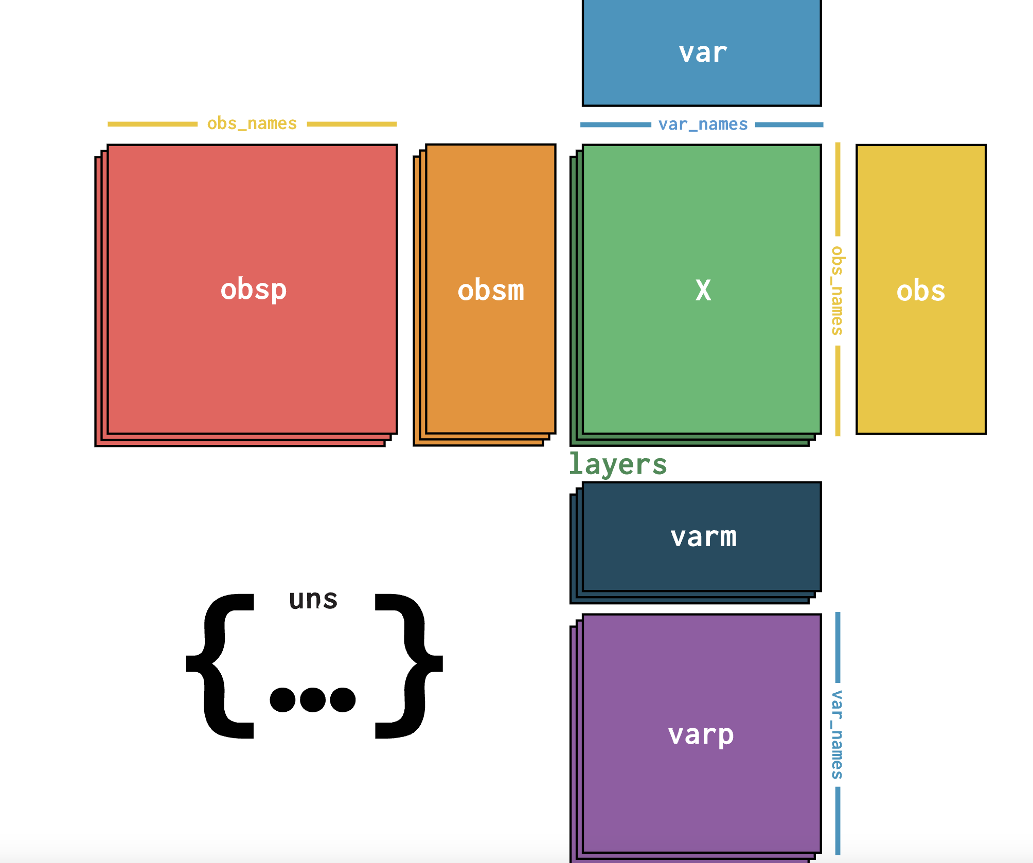
in scRNAseq data we have been fortunate to get many great python toolkits like anndata and scanpy, part of the scverse suite of tools. Allowing us to work together with a common set of standards. 📜

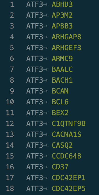
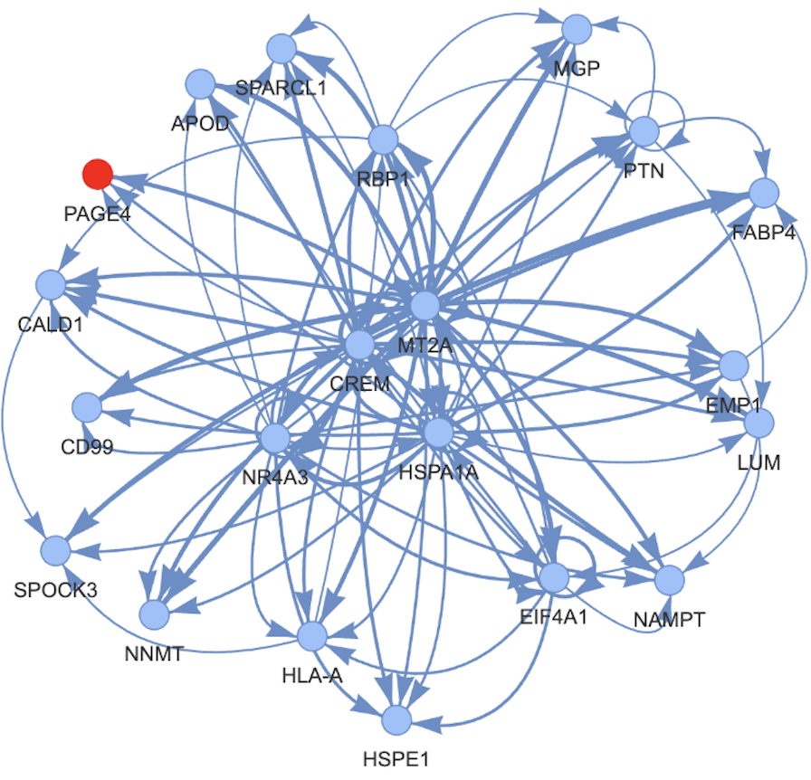
However, working with gene network methods, I have seen various ways to store them throughout the different papers and benchmarks. Often as some kind of tsv/csv/… file with some kind of a gene-gene list. This lack of standard made it quite hard for me and other members of the lab to work with gene networks 🙉

Interestingly, there is a possible standard for it! 🎉AnnData contains the .varp field which is made to store var to var (e.g. genes to gene) relationships. However not many people use it…

I thus decided to formalize this usage by creating GRnnData: it is basically a way to important many different gene-gene format to an AnnData file. 💁 But it also contains more bells and whistles to work with gene networks like subsetting the network to some genes, extracting targets, and plotting the networks 💹.

But GRnnData can do more and integrates some utils functions doing things like clustering, centrality measures, enrichment and more. Go check GRnnData if you work with gene networks!

Understanding Classification Metrics

When evaluating a binary classification model that outputs probabilities or has internal regularization, we need ways to assess its performance across different decision thresholds.

ROC Curves

One common approach is plotting the ROC curve, which shows the tradeoff between true positive and false positive rates. The area under this curve (AUC/ROC-AUC/ROC/AUROC) is a popular metric:

The Need for Precision

However, in some cases like predicting graph edges in sparse gene networks, precision becomes crucial. AUROC can miss important information about optimal cutoff points. 🚫

AUPRC and Its Challenges

This is where AUPRC (PR-AUC) becomes valuable, focusing on precision and recall:

However, AUPRC comes with its own challenges: ⚠️

1. Random precision baselines differ between tasks, making direct comparisons difficult
2. Jagged results require careful sampling of PR curves 😟
3. In gene network inference, many links lack prediction values, requiring special handling 🔥

Introducing rAUPRC

To address these limitations, I developed rAUPRC (random-baseline-corrected AUPRC), implemented in benGRN. It differs from vanilla AUPRC in three key ways:

1. Baseline correction — Standard AUPRC is heavily influenced by the positive class ratio. A dataset with 1% positives will have a baseline AUPRC of ~0.01, making comparisons across tasks meaningless. rAUPRC normalizes for this: a random classifier always scores 0, a perfect classifier scores 1, regardless of class imbalance. 🎯

2. Handling missing predictions — In gene network inference, most tools only predict a subset of possible links; the rest are simply absent (not predicted as negative). Vanilla AUPRC breaks here. rAUPRC handles this by treating missing predictions explicitly when drawing the recall axis, giving a fair picture even when coverage is partial. 🔍

3. Curve interpolation — PR curves are notoriously jagged, especially at low recall. rAUPRC uses a modified interpolation that avoids the artificial inflation that naive linear interpolation can introduce between operating points.

In practice on GRN benchmarks, rAUPRC produced more stable rankings across different network densities and prediction tool outputs than either vanilla AUPRC or AP. 📊

Average Precision (AP)

AP is computed as:

AP is a discrete approximation of AUPRC — rather than integrating the continuous curve, it sums precision at each threshold where a positive is retrieved, weighted by the change in recall:

In practice, AP and AUPRC give very similar values when the PR curve is sampled densely. The key difference is that AP is purely a summary statistic (one number per run), while AUPRC can be computed from the full curve and lends itself better to baseline correction.

AP is often recommended for object detection and ranking tasks (it’s the default in PASCAL VOC and COCO benchmarks). For gene network inference and other sparse biological tasks, rAUPRC is more appropriate. ✅

When to use what

For a deeper dive into the implementation, see the benGRN repo and the benchmarking section of the scPRINT paper.

The Decision Tree

The key question is: what shape is your data?

Enrichr — you have a gene list, nothing else

Enrichr is when you just have a list of genes (can be small). No values, no conditions — just names. 📋

GENEA, GENEB, GENEC

Under the hood, Enrichr tests each gene set in its databases using a Fisher’s exact test (hypergeometric). It asks: is my list enriched for genes in pathway X more than expected by chance?

Best for: DE gene lists, hit lists from CRISPR screens, manually curated sets.

Prerank — you have a ranked gene list

Prerank is when you have a continuous value per gene that you can rank — a fold change, a correlation, a t-statistic, anything. 📊

Prerank runs GSEA logic (the enrichment score / walking statistic) on your pre-ranked list, without needing raw expression data or phenotype labels. Useful when you already have a score but not the underlying samples.

Best for: correlation with a phenotype, output from another model, single-sample pseudo-bulk scores.

👉 Python: gseapy.prerank

GSEA — you have expression data with two conditions

GSEA works best when you have a matrix of gene expression values across multiple samples with a clear phenotype label (treated vs control, disease vs healthy, etc.). It computes its own gene ranking internally. 🔬

The key advantage over Enrichr: GSEA doesn’t require you to define a hard cutoff (“top 200 DE genes”). It uses the full ranked list and identifies pathways enriched at the top or bottom. This makes it more sensitive and less arbitrary. ✅

Best for: bulk RNA-seq, any two-condition comparison with replicates (n ≥ 3 per group recommended).

ssGSEA — you want a per-sample enrichment score

ssGSEA is for when you have many samples with no clear two-group contrast — or when you want a continuous enrichment score per sample rather than a comparison between groups. 🗂️

Each sample gets its own enrichment score for each pathway, independently. The output is a sample × pathway matrix. Great for downstream analysis — clustering, survival analysis, correlating pathway activity with other variables.

Best for: large cohorts (TCGA, GTEx), single-cell pseudo-bulk, any analysis where you want pathway activity as a continuous feature.

👉 Python: gseapy.ssgsea

Quick summary table

For most single-cell work: compute pseudo-bulk, run GSEA or Prerank per cell type. For single-cell pathway scoring directly, decoupleR is worth a look. 🔍